some Vi shortcuts

 Copy and paste one line

With the cursor at your desired line press yy. Press p wherever you like and the line will be pasted below the line you are on. The y stands for “yank”.

Cut and paste one line

With the cursor at your desired line press dd. Press p wherever you like and the line will be pasted below the line you are on. The d stands for “delete”.

Copy and paste multiple lines

With the cursor at your desired line press nyy, where n is the number of lines down you want to copy. So if you want to copy 2 lines, press 2yy. To paste press p and the number of lines copied will be pasted below the line you are on now.

Cut and paste multiple lines

With the cursor at your desired line press ndd, where n is the number of lines down you want to copy. So if you want to copy 2 lines, press 2dd. To paste press p and the number of lines copied will be pasted below the line you are on now.

Copy and paste one word in a line

Move the cursor to your desired word. It can be any part of the word and press yiw, which stands for yank inner word. Press p and your word will be pasted after the cursor.

Cut and paste one word in a line

Move the cursor to your desired word. It can be any part of the word and press diw, which stands for delete inner word. Press p and your word will be pasted after the cursor.

Copy and paste part of a word or line

Mover the cursor to your desired word. Press v, which will enter you into visual mode. Move your cursor around to highlight the words or parts of words you want to copy then press y. Press p and your selection will be pasted after the cursor.

Cut and paste part of a word or line

Mover the cursor to your desired word. Press v, which will enter you into visual mode. Move your cursor around to highlight the words or parts of words you want to cut then press d. Press p and your selection will be pasted after the cursor.

Some other commands

I think we get the pattern. Here are some other commands:

x   deletes/cuts the single character under the cursor
Nx  deletes/cuts N characters starting with the character under the cursor
dw  deletes/cuts the rest of the word the cursor is on starting with the character under the cursor
dNW deletes/cuts the N words starting with the character under the cursor
D   Delete the remainder of the line starting with the character under the cursor.

If you swicth d or x with y you get the same effect but with a copy instead of a cut. Note that Y copys the whole line not the remainder.

Ref: http://ahmed.amayem.com/copy-or-cut-and-paste-in-vi-linux-tutorial/

Why don't you see all GO terms in GSEA-MSigDB?

 This is why...

This procedure has been modified from that described previously for MSigDB v5.2. First, for each GO term we got the corresponding human genes from the gene2go file. Next, we have applied the path rule. Gene products are associated with the most specific GO terms possible. All parent terms up to the root automatically apply to the gene product. Thus, the parent GO term gene sets should include all genes associated with the children GO terms. Then we removed sets with fewer than 5 or more than 2,000 Gene IDs. Finally, we resolved redundancies as follows. We computed Jaccard coefficients for each pair of sets, and marked a pair as highly similar if its Jaccard coefficient was greater than 0.85. We then clustered highly similar sets into "chunks" using the hclust function from the R stats package according to their GO terms and applied two rounds of filtering for every "chunk". First, we kept the largest set in the "chunk" and discarded the smaller sets. This left "chunks" of highly similar sets of identical sizes, which we further pruned by preferentially keeping the more general set (i.e., the set closest to the root of the GO ontology tree).

Ref: https://software.broadinstitute.org/cancer/software/gsea/wiki/index.php/MSigDB_v5.2_Release_Notes

An easy to convert list to long table

 Say you have a list with different lengths of vectors, e.g. 

> head(genesets_list)

$KEGG_GLYCOLYSIS_GLUCONEOGENESIS

 [1] "ACSS2"   "GCK"     "PGK2"    "PGK1"    "PDHB"    "PDHA1"   "PDHA2"   "PGM2"    "TPI1"    "ACSS1"   "FBP1"    "ADH1B"   "HK2"     "ADH1C"   "HK1"     "HK3"     "ADH4"    "PGAM2"   "ADH5"    "PGAM1"   "ADH1A"   "ALDOC" "ALDH7A1" "LDHAL6B" "PKLR"    "LDHAL6A" "ENO1"    "PKM"     "PFKP"    "BPGM"    "PCK2"    "PCK1"    "ALDH1B1" "ALDH2"   "ALDH3A1" "AKR1A1"  "FBP2"    "PFKM"    "PFKL"    "LDHC"    "GAPDH"   "ENO3"    "ENO2"    "PGAM4" "ADH7"    "ADH6"    "LDHB"    "ALDH1A3" "ALDH3B1" "ALDH3B2" "ALDH9A1" "ALDH3A2" "GALM"    "ALDOA"   "DLD"     "DLAT"    "ALDOB"   "G6PC2"   "LDHA"    "G6PC"    "PGM1"    "GPI"    

$KEGG_CITRATE_CYCLE_TCA_CYCLE

 [1] "IDH3B"    "DLST"     "PCK2"     "CS"       "PDHB"     "PCK1"     "PDHA1"    "PDHA2"    "SUCLG2P2" "FH"       "SDHD"     "OGDH"     "SDHB"     "IDH3A"    "SDHC"     "IDH2"     "IDH1"     "ACO1"     "ACLY"     "MDH2" "DLD"      "MDH1"     "DLAT"     "OGDHL"    "PC"       "SDHA"     "SUCLG1"   "SUCLA2"   "SUCLG2"   "IDH3G"    "ACO2"    

$KEGG_PENTOSE_PHOSPHATE_PATHWAY

 [1] "RPE"     "RPIA"    "PGM2"    "PGLS"    "PRPS2"   "FBP2"    "PFKM"    "PFKL"    "TALDO1"  "TKT"     "FBP1"    "TKTL2"   "PGD"     "RBKS"    "ALDOA"   "ALDOC"   "ALDOB"   "H6PD"    "RPEL1"   "PRPS1L1" "PRPS1"   "DERA"  "G6PD"    "PGM1"    "TKTL1"   "PFKP"    "GPI"    

We want to convert it to a long table, with two columns (e.g. pathway ID as the first column and gene name as the 2nd column). There are various solutions (e.g. https://stackoverflow.com/questions/4227223/convert-a-list-to-a-data-frame), but none of them really works for my need. 

Martin Stingl posted a relevant solution for using map_dfr: https://rstats-tips.net/2021/02/07/converting-lists-of-lists-of-lists-to-data-frames-or-tibbles/, but didn't solve the row name problem. 

Here is my one-liner solution:

genesets_df = data.frame(pathwayID=rep(names(genesets_list), lengths(genesets_list)), geneSymbol=genesets_list %>% map_dfr(as_tibble))

Update:

An even simpler solution:

df = data.frame(ID=names(unlist(genesets_list)), geneName=unlist(genesets_list))

EASE vs. Fisher's exact test

EASE is a modified version of Fisher's exact test. It's used in DAVID. We are often asked about their difference. Here is. 

From DAVID website: https://david.ncifcrf.gov/content.jsp?file=functional_annotation.html

A Hypothetical Example 

In the human genome background (30,000 genes total; Population Total (PT)), 40 genes are involved in the p53 signaling pathway (Population Hits (PH)). A given gene list has found that three genes (List Hits (LH)) out of 300 total genes in the list (List Total (LT)) belong to the p53 signaling pathway. Then we ask the question if 3/300 is more than random chance compared to the human background of 40/30000

A 2 x 2 contingency table is built based on the above numbers: 

List Hits (LH) = 3 
List Total (LT) = 300 
Population Hits (PH) = 40 
Population Total (PT) = 30,000

Exact p-value = 0.007. Since p-value < 0.05, this user's gene list is specifically associated (enriched) in the p53 signaling pathway by more than random chance. 

What about the EASE Score 
The EASE Score is more conservative by subtracting one gene from the List Hits (LH) as seen below. If LH = 1 (only one gene in the user's list annotated to the term), EASE Score is automatically set to 1.

For our hypothetical example involving the p53 signaling pathway, the EASE Score is more conservative with a p-value = 0.06 (using 3-1 instead of 3). Since the p-value > 0.05, this user's gene list is not considered specifically associated (enriched) in the p53 signaling pathway any more than by random chance.

From https://www.ncbi.nlm.nih.gov/pmc/articles/PMC328459/:

The EASE score is offered as a conservative adjustment to the Fisher exact probability that weights significance in favor of themes supported by more genes. The theoretical basis of the EASE score lies in the concept of jackknifing a probability. The stability of any given statistic can be ascertained by a procedure called jackknifing, in which a single data point is removed and the statistic is recalculated many times to give a distribution of probabilities that is broad if the result is highly variable and tight if the result is robust [9]. The EASE score is calculated by penalizing (removing) one gene within the given category from the list and calculating the resulting Fisher exact probability for that category. It therefore represents the upper bound of the distribution of jackknife Fisher exact probabilities and has advantages in terms of penalizing the significance of categories supported by few genes. For example, assume a list of 206 genes is selected from a population of 13,679 genes. If there is only one gene in the population in some rare category, X, and that gene happens to appear on the list of 206 genes, the Fisher exact would consider category X significant (p = 0.0152). At the same time, the Fisher exact probability would deem a more common category, Y, with 787 members in the population and 20 members on the list, as slightly less significant (p = 0.0154). From the perspective of global biological themes, however, a theme based on the presence of a single gene is neither global nor stable and is rarely interesting. If the single gene happens to be a false positive, then the significance of the dependent theme is entirely false. However, the EASE score for these two situations is p = 1 for category X and p < 0.0274 for category Y, and thus the EASE score eliminates the significance of the 'unstable' category X while only slightly penalizing the significance of the more global theme Y. By extrapolating between these two extremes, the EASE score penalizes the significance of categories supported by fewer genes and thus favors more robust categories than the Fisher exact probability.

A bug related to R factor

Note a bug in my code today. Sometimes you need to put a certain level (e.g. healthy control) in the first position for your covariance. 

Here is my old code:

dds[[variable]]=factor(dds[[variable]])

levels(dds[[variable]])= union(variable_REF, levels(dds[[variable]])))

Note that this can cause problem. For example, you have two levels: HC and AD in your diagnosis. By default, setting the covariance to factor() will make the levels sorting in alphabetic order (e.g. AD then HC). In the 2nd line, if you force to change the levels to c("HC", "AD"), you are actually doing something like c(AD = "HC", HC = "AD"). This is not what you want. 

What you wanted is actually this:

dds[[variable]]=factor(dds[[variable]], levels= union(variable_REF, unique(dds[[variable]]))) 

* Too bad that blogger does not adapt to markdown language yet. 

Note (2) for DESeq2 time series data analysis

More notes on using LRT to test time-series data. Thanks for the discussion with Jie. 

1. swapping the levels of time factor won't change the LRT results, as if the time variable is a factor, LRT won't see it as a trajectory analysis but rather a factor analysis (e.g. condition-specific difference at ANY time point). 
2. subsetting only two time points {t0, ti} in LRT will get different numbers of DE genes at different time point i.  See example below; when only testing the {0, 60} minutes, 7 DE genes found. If including all time points in LRT, it will only find 4 DE genes. This could be the case that the likelihood ratio gets smaller when including time points with no or smaller condition-specific difference. Another possibility this may be happening is that there is a large dependence on t2 independent of the condition. When you add t2, you are adding it in the variable “time” to both the numerator and denominator of the LRT, and that may result in a smaller ratio.
3. converting the time covariate from a factor / categorical variable to a continuous variable can get different results. The categorical variable in LRT does not consider the slope or trajectory nature, but it can detect genes that contribute a big condition-specific difference at a specific time point while the overall slope may not change. A continuous variable can consider the slope change or trajectory analysis. It's more like a time-series analysis.  Sometimes we may need to do both. 

Note for DEseq2 time course analysis

In many cases, we need to perform differential expression across the time course data, e.g. finding genes that react in a condition-specific manner over time, compared to a set of baseline samples. DEseq2 has such an implementation for time-course experiments: 

There are a number of ways to analyze time-series experiments, depending on the biological question of interest. In order to test for any differences over multiple time points, once can use a design including the time factor, and then test using the likelihood ratio test as described in the following section, where the time factor is removed in the reduced formula. For a control and treatment time series, one can use a design formula containing the condition factor, the time factor, and the interaction of the two. In this case, using the likelihood ratio test with a reduced model which does not contain the interaction terms will test whether the condition induces a change in gene expression at any time point after the reference level time point (time 0). An example of the later analysis is provided in our RNA-seq workflow.

Below is the example in DEseq workflow using LRT to test the interaction term (e.g. any condition-specific changes at any timepoints after time 0):

http://master.bioconductor.org/packages/release/workflows/vignettes/rnaseqGene/inst/doc/rnaseqGene.html#time-course-experiments

library("fission") data("fission") ddsTC <- DESeqDataSet(fission, ~ strain + minute + strain:minute)

ddsTC <- DESeq(ddsTC, test="LRT", reduced = ~ strain + minute) resTC <- results(ddsTC)

Several notes from the DEseq2 forum:

1. By default, the result() function will return the LRT test p-value and MLE log2FC for the difference between Mut vs WT at the last timepoints, controlling for baseline
2. To get the log2FC for the difference between Mut vs WT at a different timepoint, you have to manually specify it, e.g. "strainmut.minute15" is the difference between Mut vs WT at minute 15, controlling for baseline. 
3. To generate the tables of log2 fold change of 60 minutes vs 0 minutes for the WT strain would be results(dds, name="minute_60_vs_0"); 
4. To generate the tables of log2 fold change of 60 minutes vs 0 minutes for the mut strain would be the sum of the WT term above and the interaction term which is an additional effect beyond the effect for the reference level (WT): results(dds, contrast=list(c("minute_60_vs_0","strainmut.minute60"))
5. "strainmut.minute15" is the difference between Mut vs WT at minute 15, controlling for baseline. If you add "strain_mut_vs_wt" to this, you get the LFC for Mutant vs WT at minute 15, not controlling for baseline. So the second one is the observed difference at minute 15 between the two groups (because you added in the change that was present at time=0).

Two kinds of hypothesis tests in DEseq2:

Wald test: to test if the estimated standard error of a log2 fold change is equal to zero

LRT (likelihood ratio test) between a full model and a reduced model: to test if the increased likelihood of the data using the extra terms in the full model is more than expected if those extra terms are truly zero.

compression level in samtools and gzip

samtools fastq can convert bam to fastq format, e.g. samtools fastq input.bam -o output.fastq

The output file will be automatically compressed if the file names have a .gz or .bgzf extension, e.g. 

samtools fastq input.bam -o output1.fastq.gz

Alternatively, you can also pipe the stdout to compressor explicitly, e.g.

samtools fastq input.bam | gzip > output2.fastq.gz

Interestingly, I noticed that output2.fastq.gz is significantly smaller than output1.fastq.gz, even though the uncompressed file content is the same. 

Actually, this is because of the different default compression ratios used in samtools and gzip. 

In samtools fastq, its default compression level is 1 (out of [0..9]) while gzip's default compression level is 6 (out of [1..9]). 

managing multiple SSH keys

 Let's say you have already generated an SSH key for GitHub, as instructed here:

https://docs.github.com/en/free-pro-team@latest/github/authenticating-to-github/generating-a-new-ssh-key-and-adding-it-to-the-ssh-agent

Now your .ssh folder will be like this:

PHS015945:.ssh xd010$ ll

-rw-r--r--  1 xd010  staff   165B Dec  9 23:21 config

-rw-------  1 xd010  staff   411B Dec  9 23:12 id_ed25519

-rw-r--r--  1 xd010  staff   100B Dec  9 23:12 id_ed25519.pub

where config file will be like:

Host *

  AddKeysToAgent yes

  UseKeychain yes

  IdentityFile ~/.ssh/id_ed25519

Now, you want to ssh to your HPC server without a password. You will follow instructions like this http://www.linuxproblem.org/art_9.html, e.g. 

a@A:~> ssh-keygen -t rsa
Generating public/private rsa key pair.
Enter file in which to save the key (/home/a/.ssh/id_rsa): 
Created directory '/home/a/.ssh'.
Enter passphrase (empty for no passphrase): 
Enter same passphrase again: 
Your identification has been saved in /home/a/.ssh/id_rsa.
Your public key has been saved in /home/a/.ssh/id_rsa.pub.
The key fingerprint is:
3e:4f:05:79:3a:9f:96:7c:3b:ad:e9:58:37:bc:37:e4 a@A

Now append a's new public key to b@B:.ssh/authorized_keys and enter b's password one last time:

a@A:~> cat .ssh/id_rsa.pub | ssh b@B 'cat >> .ssh/authorized_keys'
b@B's password: 

You will find that you are still asked to enter the password when you want to ssh to your HPC. Where's the problem?

How to take ultra high resolution screenshot?

This is very useful esp. when you want to use a high-resolution screenshot for a poster/printout. I currently don't find a way in Safari to save the screenshot in Responsive Mode. 

See stepwise instructions below from David Augustat's blog: https://davidaugustat.com/web/take-ultra-high-resolution-screenshots-in-chrome

Conda - A must-have for bioinformatician

As a bioinformatician, when you are given a new system (Mac, HPC, or any Linux environment), the first thing to do is probably to configure your work environment, install required tools, etc. 

Here is what I did for the new Mac:

1. This step is optional. Apple changed to default shell to zsh since the last OS. If you like bash, you can change the default zsh shell from bash:

chsh -s /bin/bash

2. Install Miniconda. Miniconda is a free minimal installer for conda, incl. only the basic ones (e.g. conda, python, zlib, etc). If you are under Linux, download the one for Linux. 

wget https://repo.anaconda.com/miniconda/Miniconda3-latest-MacOSX-x86_64.sh

bash Miniconda3-latest-MacOSX-x86_64.sh

3. Install commonly used tools with bioconda:

# update bash (the one coming with MacOS is too old)

conda install -c conda-forge bash

# samtools etc.

conda install -c bioconda samtools plink plink2

# UCSC Kent Utilities etc.

conda install -c bioconda ucsc-bedgraphtobigwig ucsc-wigtobigwig ucsc-liftover ucsc-bigwigsummary

# GNU utils etc.

conda install -c conda-forge coreutils gawk wget gzip datamash parallel make readline sed

# R and R package etc.

conda install -c r r-base

conda install -c r r-essentials

conda install -c r r-tidyverse

# Google cloud gsutil

conda install -c conda-forge gsutil 

Life is much easier after conda!

Explaination of "samtools flagstat" output

==> CRR119891.sam.flagstat <==

192013910 + 0 in total (QC-passed reads + QC-failed reads)

0 + 0 secondary

38830640 + 0 supplementary

0 + 0 duplicates

191681231 + 0 mapped (99.83% : N/A)

153183270 + 0 paired in sequencing

76591635 + 0 read1

76591635 + 0 read2

118230182 + 0 properly paired (77.18% : N/A)

152555312 + 0 with itself and mate mapped

295279 + 0 singletons (0.19% : N/A)

10160332 + 0 with mate mapped to a different chr

5532624 + 0 with mate mapped to a different chr (mapQ>=5)

Here are the notes from our careful check:

1. What's secondary, supplementary, and singleton? I was using "bwa mem" with default parameters. In that case, it only reports one alignment if the read can be mapped to multiple locations with equal quality. See discussion here: https://www.biostars.org/p/304614/#304620. That's why you don't see the secondary alignment in above example. Supplementary alignments are those alignments that are part of a chimeric alignment. For example, in a circRNA case, one read is broke into two pieces, mapped to different locations in back-splicing order. Then one of the two fragment will be supplementary (the other is not). Singleton is a mapped read whose mate is unmapped. So its flag has 0x1 and 0x8 but 0x4 is unset. Note that a singleton's mate (which is unmapped) can have a flag of 0110.  

2. What's the total number of reads? The number in the output is NOT for reads, but rather for alignment in the SAM files. The samtools flagstat only check the FLAG, not the read ID. So, in the above example, the total number of reads (R1+R2) should be 192013910 - 38830640. (If there is secondary or duplicate, it should also be excluded). It's also indicated by "paired in sequencing", 153183270 (R1 +R2). This can also be calculated by checking the read ID column e.g. cat CRR119891.sam | cut -f1 | sort -u | wc -l, then times 2 for paired-end reads.

3. How many reads are unmapped? The total alignment is sum of "mapped" + "singletons" + unmapped. So, the number of unmapped reads should be calcualted as 192013910-191681231-295279 = 37400 in above case. The unmapped reads can also be counted by checking the RNAME column in the SAM file (e.g. cat CRR119891.sam | awk '$3=="*"' | wc -l). 

4. Mappability? The above mapped % is based on "mapped" / "total" alignment, not based on reads. If for reads, it should be calculated based on above two numbers. 

Be careful of "sort -k1,1 -k2,2n -u"

When you attempted to sort and extract the unique genomic regions using "sort -k1,1 -k2,2n -u", you might make a mistake by missing the region with the same chr and start, but different end position.

The right way should be  "sort -k1,1 -k2,2n -k3,3n -u" or  "sort -k1,1 -k2,2n | sort -u"

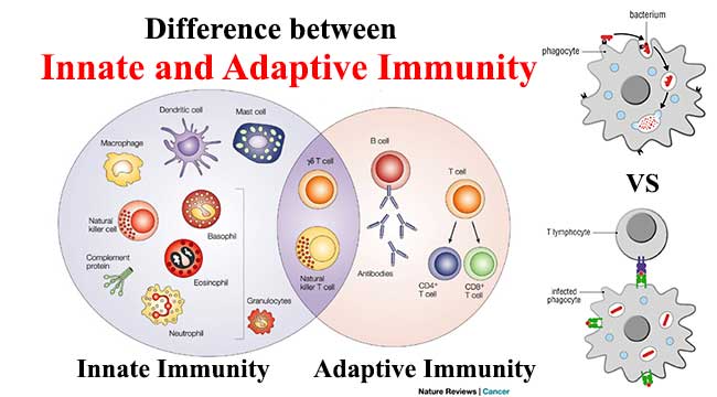
Innate vs. Adaptive Immunity

No.	Characteristics	Innate Immunity	Adaptive immunity
1.	Presence	Innate immunity is something already present in the body.	Adaptive immunity is created in response to exposure to a foreign substance.
2.	Specificity	Non-Specific	Specific
3.	Response	Fights any foreign invader	Fight only specific infection
4.	Response	Rapid	Slow (1-2 weeks)
5.	Potency	Limited and Lower potency	High potency
6.	Time span	Once activated against a specific type of antigen, the immunity remains throughout the life.	The span of developed immunity can be lifelong or short.
7.	Inheritance	Innate type of immunity is generally inherited from parents and passed to offspring.	Adaptive immunity is not passed from the parents to offspring, hence it cannot be inherited.
8.	Memory	Cannot react with equal potency upon repeated exposure to the same pathogen.	Adaptive system can remember the specific pathogens which have encountered before.
9.	Presence	Present at birth	Develops during a person’s lifetime and can be short-lived.
10.	Allergic Reaction	None	Immediate and Delay hypersensitivity
11.	Used Against	For microbes	Microbes and non-microbial substances called antigens
12.	Memory	No memory	Long term memory
13.	Diversity	Limited	High
14.	Speed	Faster response	Slower response
15.	Complement system activation	Alternative and lectin pathways	Classical pathway
16.	Anatomic and physiological barriers	Skin, Mucous membranes, Temp, pH, chemicals, etc.	Lymph nodes, spleen, mucosal associated lymphoid tissue.
17.	Composition	The innate immune system is composed of physical and chemical barriers, phagocytic leukocytes, dendritic cells, natural killer cells, and plasma proteins.	Adaptive immune system is composed of B cells and T cells.
18.	Development	Evolutionary, older and is found in both vertebrates and invertebrates.	Adaptive immunity system has been developed recently and is found only in the vertebrates.
19.	Example	White blood cells fighting bacteria, causing redness and swelling, when you have a cut.	Chickenpox vaccination so that we don’t get chickenpox because adaptive immunity system has remembered the foreign body.

Ref: https://microbiologyinfo.com/difference-between-innate-and-adaptive-immunity/

Illustrator: how to fill shapes with a 45 degree line pattern?

Reference: https://graphicdesign.stackexchange.com/a/93398

Use a pattern ...

There are a bunch of line patterns loaded with Illustrator by default (Open Swatch Library → Patterns → Basic Graphics → Basic Graphics Lines).

You can use them as a second fill using the appearance panel and use blending etc to get the effect you want. You can add a Transform effect to that specific fill (make sure to check "Transform Patterns") to get the rotation & scale you want:

...and the same with a different blending mode:

If the default line patterns don't work for you then you can, of course, make your own pattern; which should be as easy as creating a small section of the lines you want (you could do it with a single line if you really wanted to) and dragging them to the Swatches panel, then double-clicking to enter the pattern editor:

Read more here:

• How to create and edit patterns in Illustrator – Adobe Support