Notes on DEseq2 design

My note from today's lab meeting:

1. For senario like Rambo's project, where in a case-control two group comparison, each subject has multiple repeats (or multiple time points). To test the genes associated with the condition, you must model subject as a blocking factor (random effect) to properly control for within-subject correlations. DEseq2 does not take random effect directly, so we typically use linear mixed effect model from other packages like voom or dream in variancePartition for such data. Here is the correct design to linear mixed effect model wehre subjectID is a random effect:  design <- ~ group * time + age + sex + (1|subject_id) (Please note that group * time part is same as group + time + group:time where group:time is the interaction term.)
   1. If you still want to use DESeq2 (limited option), you can collapse the repeated measures by treating subject_id as a fixed effect (only works if subjects are not too many), e.g. design = ~ subjectID + age + sex + group. For case where you have many subject (e.g. usually n>20), you don't want to do that as each subjectID will become a dummy variable and it will be very computationally expensive to calculate coefficiency.
   2. Another way to test the interaction term in DEseq2 (or other similar framework) is to use LRT (likelihood ratio test) between two designs: e.g. full mode design = ~ subject_id + time + group + group:time and reduce mode as ~ subject_id + time + group , then in DEseq2, you can call function like  dds <- DESeq(dds, test="LRT", reduced = ~ subject_id + time + group) to get the genes with expression changes over time differ between groups (aka: progression-associated genes).
2. For senario like Himanshu's project, where each subject has a paired condition (e.g. before and after drug treatment, or neuroma and paired non-neuroma tissue). To test the genes associated with the condition, you can simply include the subjectID as a covariate e.g. design = ~ subjectID + age + sex + condition.

An easy to convert list to long table

 Say you have a list with different lengths of vectors, e.g. 

> head(genesets_list)

$KEGG_GLYCOLYSIS_GLUCONEOGENESIS

 [1] "ACSS2"   "GCK"     "PGK2"    "PGK1"    "PDHB"    "PDHA1"   "PDHA2"   "PGM2"    "TPI1"    "ACSS1"   "FBP1"    "ADH1B"   "HK2"     "ADH1C"   "HK1"     "HK3"     "ADH4"    "PGAM2"   "ADH5"    "PGAM1"   "ADH1A"   "ALDOC" "ALDH7A1" "LDHAL6B" "PKLR"    "LDHAL6A" "ENO1"    "PKM"     "PFKP"    "BPGM"    "PCK2"    "PCK1"    "ALDH1B1" "ALDH2"   "ALDH3A1" "AKR1A1"  "FBP2"    "PFKM"    "PFKL"    "LDHC"    "GAPDH"   "ENO3"    "ENO2"    "PGAM4" "ADH7"    "ADH6"    "LDHB"    "ALDH1A3" "ALDH3B1" "ALDH3B2" "ALDH9A1" "ALDH3A2" "GALM"    "ALDOA"   "DLD"     "DLAT"    "ALDOB"   "G6PC2"   "LDHA"    "G6PC"    "PGM1"    "GPI"    

$KEGG_CITRATE_CYCLE_TCA_CYCLE

 [1] "IDH3B"    "DLST"     "PCK2"     "CS"       "PDHB"     "PCK1"     "PDHA1"    "PDHA2"    "SUCLG2P2" "FH"       "SDHD"     "OGDH"     "SDHB"     "IDH3A"    "SDHC"     "IDH2"     "IDH1"     "ACO1"     "ACLY"     "MDH2" "DLD"      "MDH1"     "DLAT"     "OGDHL"    "PC"       "SDHA"     "SUCLG1"   "SUCLA2"   "SUCLG2"   "IDH3G"    "ACO2"    

$KEGG_PENTOSE_PHOSPHATE_PATHWAY

 [1] "RPE"     "RPIA"    "PGM2"    "PGLS"    "PRPS2"   "FBP2"    "PFKM"    "PFKL"    "TALDO1"  "TKT"     "FBP1"    "TKTL2"   "PGD"     "RBKS"    "ALDOA"   "ALDOC"   "ALDOB"   "H6PD"    "RPEL1"   "PRPS1L1" "PRPS1"   "DERA"  "G6PD"    "PGM1"    "TKTL1"   "PFKP"    "GPI"    

We want to convert it to a long table, with two columns (e.g. pathway ID as the first column and gene name as the 2nd column). There are various solutions (e.g. https://stackoverflow.com/questions/4227223/convert-a-list-to-a-data-frame), but none of them really works for my need. 

Martin Stingl posted a relevant solution for using map_dfr: https://rstats-tips.net/2021/02/07/converting-lists-of-lists-of-lists-to-data-frames-or-tibbles/, but didn't solve the row name problem. 

Here is my one-liner solution:

genesets_df = data.frame(pathwayID=rep(names(genesets_list), lengths(genesets_list)), geneSymbol=genesets_list %>% map_dfr(as_tibble))

Update:

An even simpler solution:

df = data.frame(ID=names(unlist(genesets_list)), geneName=unlist(genesets_list))

A bug related to R factor

Note a bug in my code today. Sometimes you need to put a certain level (e.g. healthy control) in the first position for your covariance. 

Here is my old code:

dds[[variable]]=factor(dds[[variable]])

levels(dds[[variable]])= union(variable_REF, levels(dds[[variable]])))

Note that this can cause problem. For example, you have two levels: HC and AD in your diagnosis. By default, setting the covariance to factor() will make the levels sorting in alphabetic order (e.g. AD then HC). In the 2nd line, if you force to change the levels to c("HC", "AD"), you are actually doing something like c(AD = "HC", HC = "AD"). This is not what you want. 

What you wanted is actually this:

dds[[variable]]=factor(dds[[variable]], levels= union(variable_REF, unique(dds[[variable]]))) 

* Too bad that blogger does not adapt to markdown language yet. 

Note (2) for DESeq2 time series data analysis

More notes on using LRT to test time-series data. Thanks for the discussion with Jie. 

1. swapping the levels of time factor won't change the LRT results, as if the time variable is a factor, LRT won't see it as a trajectory analysis but rather a factor analysis (e.g. condition-specific difference at ANY time point). 
2. subsetting only two time points {t0, ti} in LRT will get different numbers of DE genes at different time point i.  See example below; when only testing the {0, 60} minutes, 7 DE genes found. If including all time points in LRT, it will only find 4 DE genes. This could be the case that the likelihood ratio gets smaller when including time points with no or smaller condition-specific difference. Another possibility this may be happening is that there is a large dependence on t2 independent of the condition. When you add t2, you are adding it in the variable “time” to both the numerator and denominator of the LRT, and that may result in a smaller ratio.
3. converting the time covariate from a factor / categorical variable to a continuous variable can get different results. The categorical variable in LRT does not consider the slope or trajectory nature, but it can detect genes that contribute a big condition-specific difference at a specific time point while the overall slope may not change. A continuous variable can consider the slope change or trajectory analysis. It's more like a time-series analysis.  Sometimes we may need to do both. 

Note for DEseq2 time course analysis

In many cases, we need to perform differential expression across the time course data, e.g. finding genes that react in a condition-specific manner over time, compared to a set of baseline samples. DEseq2 has such an implementation for time-course experiments: 

There are a number of ways to analyze time-series experiments, depending on the biological question of interest. In order to test for any differences over multiple time points, once can use a design including the time factor, and then test using the likelihood ratio test as described in the following section, where the time factor is removed in the reduced formula. For a control and treatment time series, one can use a design formula containing the condition factor, the time factor, and the interaction of the two. In this case, using the likelihood ratio test with a reduced model which does not contain the interaction terms will test whether the condition induces a change in gene expression at any time point after the reference level time point (time 0). An example of the later analysis is provided in our RNA-seq workflow.

Below is the example in DEseq workflow using LRT to test the interaction term (e.g. any condition-specific changes at any timepoints after time 0):

http://master.bioconductor.org/packages/release/workflows/vignettes/rnaseqGene/inst/doc/rnaseqGene.html#time-course-experiments

library("fission") data("fission") ddsTC <- DESeqDataSet(fission, ~ strain + minute + strain:minute)

ddsTC <- DESeq(ddsTC, test="LRT", reduced = ~ strain + minute) resTC <- results(ddsTC)

Several notes from the DEseq2 forum:

1. By default, the result() function will return the LRT test p-value and MLE log2FC for the difference between Mut vs WT at the last timepoints, controlling for baseline
2. To get the log2FC for the difference between Mut vs WT at a different timepoint, you have to manually specify it, e.g. "strainmut.minute15" is the difference between Mut vs WT at minute 15, controlling for baseline. 
3. To generate the tables of log2 fold change of 60 minutes vs 0 minutes for the WT strain would be results(dds, name="minute_60_vs_0"); 
4. To generate the tables of log2 fold change of 60 minutes vs 0 minutes for the mut strain would be the sum of the WT term above and the interaction term which is an additional effect beyond the effect for the reference level (WT): results(dds, contrast=list(c("minute_60_vs_0","strainmut.minute60"))
5. "strainmut.minute15" is the difference between Mut vs WT at minute 15, controlling for baseline. If you add "strain_mut_vs_wt" to this, you get the LFC for Mutant vs WT at minute 15, not controlling for baseline. So the second one is the observed difference at minute 15 between the two groups (because you added in the change that was present at time=0).

Two kinds of hypothesis tests in DEseq2:

Wald test: to test if the estimated standard error of a log2 fold change is equal to zero

LRT (likelihood ratio test) between a full model and a reduced model: to test if the increased likelihood of the data using the extra terms in the full model is more than expected if those extra terms are truly zero.

Making Art in R

Amazing artworks people made in R:

See their source code and more arts at:
http://www.r-graph-gallery.com/286-antonio-sanchez-dataart/

More about generative arts in R here:

https://daljitsdatadistractions.wordpress.com/2019/10/11/automated-artistry-making-art-with-r/

PCA plot with fill, color, and shape all together

When I plotted the PCA results (e.g. scatter plot for PC1 and PC2) and was about to annotate the dataset with different covariates (e.g. gender, diagnosis, and ethic group), I noticed that it's not straightforward to annotate >2 covariates at the same time using ggplot.

Here is what works for me in ggplot:

pcaData <- plotPCA(vsd, intgroup = c( "Diagnosis", "Ethnicity", "Sex"), returnData = TRUE) # vsd and plotPCA are part of DESeq2 package, nothing with my example below. 

percentVar <- round(100 * attr(pcaData, "percentVar")) 

ggplot(pcaData, aes(x = PC1, y = PC2, color = factor(Diagnosis), shape = factor(Ethnicity))) + 

geom_point(size =3, aes(fill=factor(Diagnosis), alpha=as.character(Sex))) + 

geom_point(size =3) + 

scale_shape_manual(values=c(21,22)) + 

scale_alpha_manual(values=c("F"=0, "M"=1)) + 

xlab(paste0("PC1: ", percentVar[1], "% variance")) + 

ylab(paste0("PC2: ", percentVar[2], "% variance")) + 

ggtitle("PCA of all genes, no covariate adjusted")

I also found that you can use the male and female symbol (♂ ♀) as shapes in your plot. Here is how:

df <- data.frame(x = runif(10), y = runif(10), sex = sample(c("m","f"), 10, rep = T)) 

qplot(x, y, data = df, shape = sex, size = I(5)) + 

scale_shape_manual(values = c("m" = "\u2642", f = "\u2640"))

(Reference: https://github.com/kmiddleton/rexamples/blob/master/ggplot2%20male-female%20symbols.R)

I've not figured out a way to combine the two ideas above.

Download all KEGG pathway KGML files for SPIA analysis

Most people know the KEGG pathway, but not everyone knows that it costs at least $2000 to subscribe to its database. If you want to save the cost a bit, you can manually download the KEGG pathway KGML files and install them in SPIA. Here I have a workaround to download all KEGG pathway files using their REST API.
## Claim: this is my personal trick. I recommend people subscribe to their KEGG FTP download to support the authors.

# change folder to the folder where your SPIA installed, for example in my Mac
cd /Library/Frameworks/R.framework/Versions/4.0/Resources/library/SPIA
# download all XML and png files for all human pathway
curl -s http://rest.kegg.jp/list/pathway/hsa | awk '{split($1,a,":"); print "curl -s http://rest.kegg.jp/get/"a[2]"/kgml -o extdata/keggxml/hsa/"a[2]".xml"}' | bash

curl -s http://rest.kegg.jp/list/pathway/hsa | awk '{split($1,a,":"); print "curl -s http://rest.kegg.jp/get/"a[2]"/image -o extdata/keggxml/hsa/"a[2]".png"}' | bash

# then switch to R console
setwd("/Library/Frameworks/R.framework/Versions/3.4/Resources/library/SPIA")
library(SPIA)
makeSPIAdata(kgml.path=system.file("extdata/keggxml/hsa",package="SPIA"),organism="hsa",out.path="./extdata")

Done!

Best way to draw heatmap for publication

Here are two tips I can share if you were also working on a big dataset towards a high quality heatmap:

1. Don't generate PDF using pheatmap() or heatmap.2() as (i) the file is unnecessarily SUPER large if you have a lot of data points in the heatmap, so that you can kill your Illustrator; (ii) annoying grey boxes added to the grip (see here). Use basic image() with zero margins (e.g. par(mar=c(0,0,0,0))) to generate high-resolution PNG (or JPEG, TIFF) and place in Adobe Illustrator. You can freely add legend/annotation there easily.

2. When you use image(), rotate your matrix 90 degree clockwise first, so that the conventional printed layout of the matrix is same what you see in the image (e.g. top-left corner --> x(1,1) in your matrix etc.). An elegant piece of code for clockwise rotation can be found here:

rotate <- function(x) t(apply(x, 2, rev))

My 15 practical tips for a bioinformatician

Tips below are based on the lessons I learnt from making mistakes during my years of research. It's purely personal opinion. Order doesn't mean anything. If you think I should include something else, please comment below.

1. Always set a seed number when you run tools with random option, e.g. bedtools shuffle, random etc.; You (or your boss in a day) want your work reproducible. 
2. Set your own temporary folder (via --tmp, $TMPDIR etc., depending on your program). By default, many tools, e.g. sort, use the system /tmp as temporary folder, which may have limited quote that is not enough for your big NGS data. 
3. Always use a valid name for your variables, column and rows of data frame. Otherwise, it can bring up unexpected problem, e.g. a '-' in the name will be transferred to '.' in R unless you specify check.names=F.
4. Always make a README file for the folder of your data; For why and how, read this: http://stackoverflow.com/questions/2304863/how-to-write-a-good-readme
5. Always comment your code properly, for yourself and for others, as you very likely will read your ugly code again.
6. Always backup your code timely, using github, svn, Time Machine, or simply copy/paste whatever.
7. Always clean up the intermediate or unnecessary data, as you can easily shock your boss and yourself by generating so much data (and perhaps most of them are useless). 
8. Don't save into *.sam if you can use *.bam. Always zip your fastq (and other large plain files) as much as you. This applies to other file format if you can use the compressed one. As you cannot imagine how much data (aka "digital garbage") you will generate soon.
9. Using parallel as much as you can, e.g. using "LC_ALL=C sort --parallel=24 --buffer-size=5G" for sorting (https://www.biostars.org/p/66927/), as multi-core CPU/GPU is common nowaday.
10. When a project is completed, remember to clean up your project folder, incl. removing the unnecessary code/data/intermediate files, and burn a CD or host it somewhere in cloud for the project. You never know when you, your boss or your collaborators will need the data again;
11. Make your code sustainable as possible as you can. Remember the 3 major features of OOP: Inheritance, Encapsulation, Polymorphism. (URL)
12. When you learn some tips from others by Google search, remember to list the URL for future reference and also for acknowledging others' credit. This applies to this post, of course :)
13. Keep learning, otherwise you will be out soon. Just like the rapid development of NGS techniques, computing skills are also evolving quickly. Always catch up with the new skills/tools/techniques.
14. When you learn some tips from others, remember to share something you learned to the community as well, as that's how the community grows healthily. 
15. Last but not least, stand up and move around after sitting for 1-2 hours. This is especially important for us bioinformaticians who usually sit in front of computer for hours. Only good health can last your career long. More reading: https://www.washingtonpost.com/news/wonk/wp/2015/06/02/medical-researchers-have-figured-out-how-much-time-is-okay-to-spend-sitting-each-day/

Calculate the odd of winning Powerball in R

This Wednesday’s Powerball grand prize already climbed up to $1.5 BILLION. If you choose to cash out, it would be $930 million. And it keeps increasing…
So, what’s the odd of winning the jackpot prize?
Here is the game rule according to Powerball.com:

…we draw five white balls out of a drum with 69 balls and one red ball
out of a drum with 26 red balls.

We can calculate the total number of different combinations in R:

> choose(69,5)*26
[1] 292201338

If we are super super lucky to win the Jackpot of $930 million cash value, given that we have to pay 39.6% as federal tax, how much we expect to return for a $2 investment? (Of course, everyone expect to win the $1.5 billion jackpot)

> 930e6*(1-0.396)/(choose(69,5)*26)
[1] 1.92

Actually it’s not a good investment. (Thanks for the comment below. I made a mistake; 930million should be 930e6, not 930e9).
If we want to be 100% guaranteed, we have to buy all 292 million combinations. In that case, can we earn?

# this is what we pay
> choose(69,5)*26*2
[1] 584,402,676

# this is what we earn in total, before tax
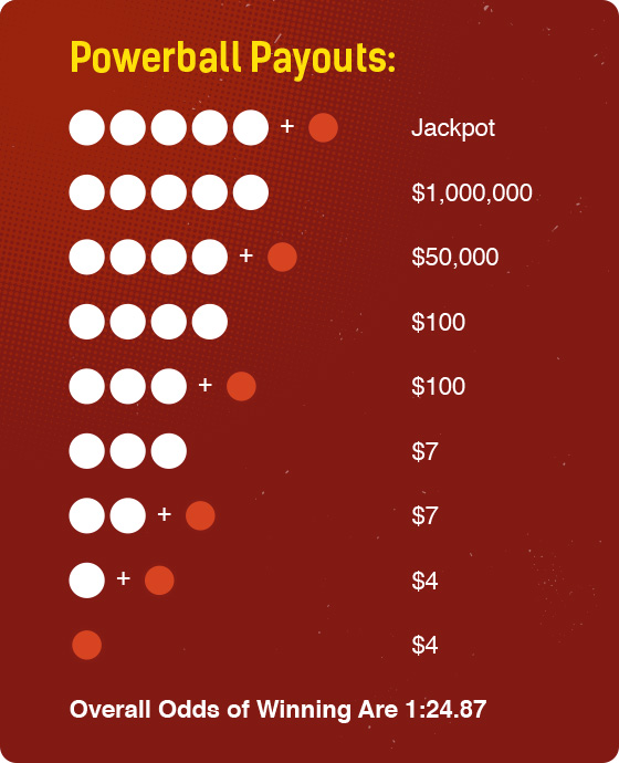
> 930000000 + 1000000*choose(25,1) + 50000*choose(5,4)*choose(69-5,1) + 100*choose(5,4)*choose(69-5,1)*choose(25,1) + 100*choose(5,3)*choose(69-5,2) + 7*choose(5,3)*choose(69-5,2)*choose(25,1) + 7*choose(5,2)*choose(69-5,3) + 4*choose(5,1)*choose(69-5,4) + 4*choose(69-5,5)
[1] 1,023,466,048

# Nearly $5 billion!!! Then we need to pay 40% of tax. Maybe not for the minor prize, let's simplify it for all.
> 1023466048 * (1-0.396)
[1] 618,173,493

That’s still more than what we paid. Why don’t we do that?
Remember, people share the prize if multiple persons got the same winning number, which we don’t know. :D

Just some fun! :)

---

References:
1. Fascinating Math Behind Why You Won’t Win Powerball
(http://www.wired.com/2016/01/the-fascinating-math-behind-why-you-wont-win-powerball/)
2. Tax for lottery (http://classroom.synonym.com/much-federal-taxes-held-lottery-winnings-20644.html)

My note on multiple testing

It's not a shame to put a note on something (probably) everyone knows and you thought you know but actually you are not 100% sure. Multiple testing is such a piece in my knowledge map.

Some terms first:
- Type I error (false positive) and Type II error (false negative): 
When we do a hypothesis test, we can categorize the result into the following 2x2 table:

Table of error types		Null hypothesis (H0) is
		Valid/True	Invalid/False
Judgement of Null Hypothesis (H0)	Reject	Type I error (False Positive)	Correct inference (True Positive)
	Fail to reject	Correct inference (True Negative)	Type II error (False Negative)

Type I error is "you reject a true thing". If the true thing is a null hypothesis (H0), which is what people usually assume (e.g. no difference, no effect), then you reject it (or yes, there is difference), it's like a false positive. The similar logics for Type II error, or false negative.

Also note that people use Greek letter α for type I error rate and β for type II error rate. α is also the significant level for a test, e.g. 5%. So when a single test reaches p-value 0.05, we can intuitively understand that with 5% of chance we make a mistake or 5% of cases we thought significant are actually not. β is related with the power of a test. Power of a test = the ability to detect True Positive among all real positive cases.

- Sensitivity and Specificity

Total test (m)		Null hypothesis (H0) is
		Valid/True	Invalid/False
Judgement of Null Hypothesis (H0)	Reject (R)	V	S
	Fail to reject	U	T

Sensitivity = S / (S+T)  = power = 1-β
Specificity = U / (U+V) = 1-α

- Why multiple testing matters?
It matters because we usually perform the same hypothesis tests not just once, but many many times. If your chance of making an error in single test is α, then your chance to make one or more errors in m tests will be

Pr(at least one error)=1−(1−α)^m

So, then m is large, the chance will be nearly 100%. That's why we need to adjust the p-values for the number of hypothesis tests performed, or to control type I error rate.

- How to control type I error rate in multiple test?

There are many different ways to control the type I errors, such as
Per comparison error rate (PCER): the expected value of the number of Type I errors over the number of hypotheses, PCER = E(V)/m
Per-family error rate (PFER): the expected number of Type I errors, PFE = E(V).
Family-wise error rate (FWER): the probability of at least one type I error, FWER = P(V ≥ 1)
False discovery rate (FDR) is the expected proportion of Type I errors among the rejected hypotheses, FDR = E(V/R | R>0)P(R>0)
Positive false discovery rate (pFDR): the rate that discoveries are false, pFDR = E(V/R | R > 0)

- Controlling Family-Wise Error Rate
Many procedures have been developed to control the family-wise error rate P(V≥ 1), including the Bonferroni, Holm (1979), Hochberg (1988), and Sidak. It consists of two types: single-step (e.g. Bonferroni) and sequential adjustment (e.g. Holm or Hochberg). Bonferroni correction is to control the overall type I errors when all tests are independent. It rejects any hypothesis with p-value ≤ α/m. So, when doing corrections, simply multiply the nominal p-value by m to get the adjusted p-values. In R, it's the following function

p.adjust(p, method = "bonferroni")

The sequential corrections is slightly more powerful than Bonferroni test. The Holm step-down procedure is the easiest to understand. First, sort your thousand p-values from low to high. Multiply the smallest p-value by one thousand. If that adjusted p-value is less than 0.05, then that gene shows evidence of differential expression. There is no difference as Bonferroni test for the gene. Then for the 2nd one, multiply its p-value by 999 (not one thousand) and see if it is less than 0.05. Multiply the third smallest p-value by 998, the fourth smallest by 997, etc. Compare each of these adjusted p-values to 0.05. We then insure that any adjusted p-value is at least as large as any preceding adjusted p-value. If it is not make sure it is equal to the largest of the preceding p-values. This is the algorithm of Holm step-down procedure. In R, it's

p.adjust(p, method = "holm")

- Controlling FDR

FWER is appropriate when you want to guard against ANY false positives. However, in many cases (particularly in genomics) we can live with a certain number of false positives. In these cases, the more relevant quantity to control is the false discovery rate (FDR). False discovery rate (FDR) is designed to control the proportion of false positives (V) among the set of rejected hypotheses (R). The FDR control has generated a lot of interest due to its more balanced trade-off between error rate control and power than the traditional Family-wise Error Rate control

Procedures controlling FDR include Benjamini & Hochberg (1995), Benjamini & Yekutieli (2001), Benjamini & Hochberg (2000) and two-stage Benjamini & Hochberg (2006).

Here are the steps for Benjamini & Hochberg FDR:

1. sort nominal p-values from small to big: p1 ≤ p2 ≤ … ≤ pm

2. find a highest rank of j with pj < (j/m) x δ, where δ is the controlled FDR level. 

3. declare the tests of rank 1, 2, …, j as significant, and their adjusted p-values as pj*m/j. 

Reference:

http://www.r-bloggers.com/adjustment-for-multiple-comparison-tests-with-r-resources-on-the-web/

http://www.gs.washington.edu/academics/courses/akey/56008/lecture/lecture10.pdf

http://www.stat.berkeley.edu/~mgoldman/Section0402.pdf

How to correctly set color in the image() function?

Sometimes we want to make our own heatmap using image() function. I recently found it's tricky to set the color option there, as its manual has very little information on col:

I posted my question on BioStars. The short answer is: Unless the breaks is set, the range of Z is evenly cut into N intervals (where N = the length of color) and values in Z are assigned to the color of corresponding interval.

For example, when x=c(3,1,2,1) and col=c("blue","red",'green','yellow'), the minimal of x is assigned as the first color, and max to the last color. Any value between is calculated proportionally to a color. In this case, 2 is the the middle one, according to the principal that intervals are closed on the right and open on the left, it's assigned to "red". So, that's why we see the colors are yellow-->blue-->red-->blue.

x=c(3,1,2,1)

image(1,1:length(x), matrix(x, nrow=1, ncol=length(x)), col=c("blue","red",'green','yellow'))

In practice, unless we want to manually define the color break points, we just set the first and last color, it will automatically find colors for the values in Z.

collist<-c(0,1)
image(1:ncol(x),1:nrow(x), as.matrix(t(x)), col=collist, asp=1)

If we want to manually define the color break points, we need to

x=matrix(rnorm(100),nrow=10)*100
xmin=0; xmax=100;
x[x<xmin]=xmin; x[x>xmax]=xmax;
collist<-c("#053061","#2166AC","#4393C3","#92C5DE","#D1E5F0","#F7F7F7","#FDDBC7","#F4A582","#D6604D","#B2182B","#67001F")
ColorRamp<-colorRampPalette(collist)(10000)
ColorLevels<-seq(from=xmin, to=xmax, length=10000)
ColorRamp_ex <- ColorRamp[round(1+(min(x)-xmin)*10000/(xmax-xmin)) : round( (max(x)-xmin)*10000/(xmax-xmin) )]
par(mar=c(2,0,2,0), oma=c(3,3,3,3))
layout(matrix(seq(2),nrow=2,ncol=1),widths=c(1),heights=c(3,0.5))
image(t(as.matrix(x)), col=ColorRamp_ex, las=1, xlab="",ylab="",cex.axis=1,xaxt="n",yaxt="n")
image(as.matrix(ColorLevels),col=ColorRamp, xlab="",ylab="",cex.axis=1,xaxt="n",yaxt="n")
axis(1,seq(xmin,xmax,10),seq(xmin,xmax,10))

Tips and Tools you may need for working on BIG data

Nowadays everyone is talking about big data. As a genomic scientist, I could feel hungry of a collection of tools more specialized for the mediate-to-big data we deal everyday.

Here are some tips I found useful when getting, processing or visualizing large data set:

1. How to download data faster than wget?

We can use wget to download the data to local disk. If it's large, we can download with other faster alternative, such as axel, aria2.

http://www.cyberciti.biz/tips/download-accelerator-for-linux-command-line-tools.html

2. Process the data in parallel with hidden option in GNU commands

• If you have many many files to process, and they are independent, you can process them in a parallel manner. GNU has a command called parallel. Lindenbaum Pierre wrote a nice notebook for "GNU Parallel in Bioinformatics", worthy to read. 
• Many commonly used commands also have a hidden option to run in a parallel way. For example, GNU sort command has --parallel=N to set it with multiple cores. 
• You can set -F when doing grep -f on a large seed file. People also suggest to set export LC_ALL=C line to get X2 speed.

3. In R, there are several must-have tips for large data, e.g. data.table

• If using read.table(), set stringsAsFactors = F and colClass. See the example here. 
• use fread(), not read.table(). Some more details here. But so far, fread() does not support reading *.gz file directly. Use fread('zcat file.gz')
• use data.table, rather data.frame. Learn the difference online here.
• There is a nice View for how to process data in parallel in R: http://cran.r-project.org/web/views/HighPerformanceComputing.html, but I have not followed them practically. Hopefully there will be some easy tutorials there, or I become less procrastinated to learn some of them ... At least I can start with foreach()
• http://stackoverflow.com/questions/1727772/quickly-reading-very-large-tables-as-dataframes-in-r

4. How to open scatter plot with too many points in Illustrator?

This is really a problem for me as we usually have a figure with >30k dots (i.e. each dot is a gene). Even though they are highly overlapping each other, opening it in Illustrator is extremely slow. Here is a tip: http://tex.stackexchange.com/questions/39974/problem-with-a-very-heavy-eps-image-scatter-plot-too-heavy-as-eps
From that, probably a better idea is to "compress" the data before plotting it, such as merge the overlapped ones if they overlapped some %.
or this one:
http://stackoverflow.com/questions/18852395/writing-png-plots-into-a-pdf-file-in-r
or this one:
http://stackoverflow.com/questions/7714677/r-scatterplot-with-too-many-points

Still working on the post...

X11 connection error in Mac

Typically, I log into my remote server/cluster via "ssh -X" and from there launch R program for plotting. But it always shows an error as

unable to open connection to X11 display ''

after a while, when you want to call functions such as plot(). 

This is very annoying. So that I have to exit the server and re-login again. 

Does this sound familiar for you?

Here is the solution I found via website below:

http://b.kl3in.com/2012/01/x11-display-forwarding-fails-after-some-time/

Two ways to solve this:

1. add the following line to the Mac client’s /etc/ssh_config:

ForwardX11Timeout 596h
2. use “ssh -Y <remote system>”, instead of -X, as it may not trigger the untrusted auth timeout.

reshape: from long to wide format

This is to continue on the topic of using the melt/cast functions in reshape to convert between long and wide format of data frame. Here is the example I found helpful in generating covariate table required for PEER (or Matrix_eQTL) analysis:

Here is my original covariate table:

Let's say we need to convert the categorical variables such as condition, cellType, batch, replicate, readLength, sex into indicators (Note: this is required by most regression programs like PEER or Matrix-eQTL, since for example the batch 5 does not match it's higher than batch 1, unlike the age or PMI). So, we need to convert this long format into wide format. Here is my R code for that:

library(reshape2)

categorical_varaibles = c("batch", "sex", "readsLength", "condition", "cellType", "replicate");

for(x in categorical_varaibles) {cvrt = cbind(cvrt, value=1); cvrt[,x]=paste0(x,cvrt[,x]); cvrt = dcast(cvrt, as.formula(paste0("... ~ ", x)), fill=0);}

Here is output:

vennpieR: combination of venn diagram and pie chart in R

I was wondering how to draw a venn diagram like pie chart in R, to show the distribution of my RNA-seq reads mapped onto different annotation regions (e.g. intergenic, intron, exons etc.). A google search returns several options, including the nice one from Xiaopeng's bam2x (see below). However, he told me it's not released yet. And it's javascript based.

Why not I just make one in R? 

Here is the design scratch:

And here is example code:

Here is output:

You can also use par(mfrow=c(n,m)) to put multiple venn pieagram in one figure. 

reshape2: convert table from wide to long format

I found this elegant note about reshape2 from Sean Anderson's blog:
http://seananderson.ca/2013/10/19/reshape.html

Basically,

reshape2 is based around two key functions: melt and cast:
melt takes wide-format data and melts it into long-format data.
cast takes long-format data and casts it into wide-format data.

For example, this is wide format:

> head(fpkm)

ID                  FPKM.SRR1069188 FPKM.SRR1070986 FPKM.SRR1071289

ENSG00000240361.1      1.00000000        1.000000        1.000000

ENSG00000186092.4      1.00000000        1.000000        1.000000

ENSG00000237613.2      1.00000000        1.000000        1.000000

ENSG00000239906.1      0.05888838        5.139312        5.055983

ENSG00000241860.1      1.20237363        1.160175        1.085992

ENSG00000222623.1      1.00000000        1.000000        1.000000

Using melt to change it into long format:

>require('reshape2')

>head(melt(fpkm))

No id variables; using all as measure variables

         variable      value

1 FPKM.SRR1069188 1.00000000

2 FPKM.SRR1069188 1.00000000

3 FPKM.SRR1069188 1.00000000

4 FPKM.SRR1069188 0.05888838

5 FPKM.SRR1069188 1.20237363

6 FPKM.SRR1069188 1.00000000

or, you can set the column name by

> head(melt(fpkm, variable.name = "Sample",value.name ="FPKM"))

No id variables; using all as measure variables

           Sample       FPKM

1 FPKM.SRR1069188 1.00000000

2 FPKM.SRR1069188 1.00000000

3 FPKM.SRR1069188 1.00000000

4 FPKM.SRR1069188 0.05888838

5 FPKM.SRR1069188 1.20237363

6 FPKM.SRR1069188 1.00000000

if you want, you can also keep some of columns as ID in the long format, for example, I want to keep the gene ID in the long format:

>head(melt(fpkm, variable.name = "Sample",value.name ="FPKM", id="ID"))

                 ID          Sample       FPKM

1 ENSG00000240361.1 FPKM.SRR1069188 1.00000000

2 ENSG00000186092.4 FPKM.SRR1069188 1.00000000

3 ENSG00000237613.2 FPKM.SRR1069188 1.00000000

4 ENSG00000239906.1 FPKM.SRR1069188 0.05888838

5 ENSG00000241860.1 FPKM.SRR1069188 1.20237363

6 ENSG00000222623.1 FPKM.SRR1069188 1.00000000

I will do the long-->wide example when I have a good case to show... :)

Update: see this post of the long-->wide conversion. 

Access Google Spreadsheet directly in bash and in R

Google Doc is a good way to share/manage documents between you and your colleagues, but sometime you want to directly access the data in terminal (e.g. bash) or in program (e.g. R), without downloading the data first.

For example, I have a Google Spreadsheet here:

https://docs.google.com/spreadsheet/pub?key=0Aumm3V3g3dF7dFR6eWRJQjE0UHJpdU8yVTlxb2hUMFE

I want to open it in R or select some of columns in bash. Here are the tips for that:

Step1: publish the tab you want to access to the web [howto], in format of CVS or TXT (which is a tab-delimited file actually)

Step2: copy the published URL. At the end, you will see "&output=txt" part for output format, and "&gid=0" to indicate which tab to access (if you have multiple tab, specify tab number here, which starts from 0).

Step3: To access the file externally. Done.

For example, to access the 1st and 3rd columns in bash:

wget --no-check-certificate -q -O - 'https://docs.google.com/spreadsheet/pub?key=0Aumm3V3g3dF7dFR6eWRJQjE0UHJpdU8yVTlxb2hUMFE&single=true&gid=0&output=txt' | cut -f1,3

or
curl -s 'https://docs.google.com/spreadsheet/pub?key=0Aumm3V3g3dF7dFR6eWRJQjE0UHJpdU8yVTlxb2hUMFE&single=true&gid=0&output=txt'

Note: the quote on the URL is a must.
In R,

myURL="https://docs.google.com/spreadsheet/pub?key=0Aumm3V3g3dF7dFR6eWRJQjE0UHJpdU8yVTlxb2hUMFE&gid=0&output=tsv"
require(RCurl)
myTable=read.delim(textConnection(getURL(myURL)))

Note: the above code still works as a simple solution. Just note that Google has changed the txt into tsv, as I highlighted above (2016-Feb-2)

How to see source code of a function/method in R?

If it's an internal function of R (e.g. from base package), just type the function name, like

> rowMeans

function (x, na.rm = FALSE, dims = 1L) 

{

    if (is.data.frame(x)) 

        x <- as.matrix(x)

    if (!is.array(x) || length(dn <- dim(x)) < 2L) 

        stop("'x' must be an array of at least two dimensions")

    if (dims < 1L || dims > length(dn) - 1L) 

        stop("invalid 'dims'")

    p <- prod(dn[-(1L:dims)])

    dn <- dn[1L:dims]

    z <- if (is.complex(x)) 

        .Internal(rowMeans(Re(x), prod(dn), p, na.rm)) + (0+1i) * 

            .Internal(rowMeans(Im(x), prod(dn), p, na.rm))

    else .Internal(rowMeans(x, prod(dn), p, na.rm))

    if (length(dn) > 1L) {

        dim(z) <- dn

        dimnames(z) <- dimnames(x)[1L:dims]

    }

    else names(z) <- dimnames(x)[[1L]]

    z

}

<bytecode: 0x111390028>

<environment: namespace:base>

If it's a S4 function in a package, e.g. to see the code of plotMA in the DESeq2 package, first find the object it belongs to using showMethods(), like

> showMethods('plotMA')

Function: plotMA (package BiocGenerics)

object="ANY"

object="character"

    (inherited from: object="ANY")

object="DESeqDataSet"

then to get source code by getMethod(), 

> getMethod("plotMA","DESeqDataSet")

Method Definition:

function (object, ...) 

{

    .local <- function (object, lfcColname, pvalues, pvalCutoff = 0.1, 

        ylim, linecol = "#ff000080", pointcol = c("black", "red"), 

        xlab, ylab, log = "x", cex = 0.45, ...) 

    {

        if (missing(xlab)) 

            xlab <- "mean of normalized counts"

        if (missing(ylab)) 

            ylab <- expression(log[2] ~ fold ~ change)

        if (!missing(pvalues)) {

            if (length(pvalues) != nrow(object)) {

                stop("length of pvalues should be equal to the number of rows of object")

            }

        }

        stopifnot(length(pointcol) == 2)

        if (!"results" %in% mcols(mcols(object))$type) {

            stop("first run DESeq() in order to produce an MA-plot")

        }

        if (missing(lfcColname)) {

            lfcColname <- lastCoefName(object)

        }

        if (length(lfcColname) != 1 | !is.character(lfcColname)) {

            stop("the argument 'lfcColname' should be a character vector of length 1")

        }

        if (missing(pvalues)) {

            res <- results(object, name = lfcColname)

            pvalues <- res$padj

        }

        x <- mcols(object)

        stopifnot(length(cex) == 1)

        col <- ifelse(is.na(pvalues) | pvalues > pvalCutoff, 

            pointcol[1], pointcol[2])

        col = col[x$baseMean > 0]

        x = x[x$baseMean > 0, ]

        py = x[, lfcColname]

        if (missing(ylim)) 

            ylim = c(-1, 1) * quantile(abs(py[is.finite(py)]), 

                probs = 0.99) * 1.1

        plot(x$baseMean, pmax(ylim[1], pmin(ylim[2], py)), log = log, 

            pch = ifelse(py < ylim[1], 6, ifelse(py > ylim[2], 

                2, 20)), cex = cex, col = col, xlab = xlab, ylab = ylab, 

            ylim = ylim, ...)

        abline(h = 0, lwd = 4, col = linecol)

    }

    .local(object, ...)

}

<environment: namespace:DESeq2>

Signatures:

        object        

target  "DESeqDataSet"

defined "DESeqDataSet"

Reference: http://stackoverflow.com/questions/5937832/r-show-source-code-of-an-s4-function-in-a-package