How to select MACS peaks based on p-value, fold_enrichment and FDR?

In the output peaks.xls file from MACS(v1.4), there are 3 columns: -10log10(pvalue), fold_enrichment, and FDR(%). We can use these three columns to sort/filter peaks. Here are what they means:

The '−10*log10(Pvalue)' column lists the transformed P value of each peak, which makes peak sorting easier. For example, a P value of 1e−5 would be transformed to 50. The 'fold_enrichment' column shows the ratio of the ChIP-seq read count to the local value of lambda within each peak. The 'FDR(%)' column contains the empirical FDR percentage for each peak. For example, the fourth peak in the list has an 'FDR(%)' value of '6.45' and '−10*log10(Pvalue)' value of '83.67'; using the same P value cutoff of 4.4e−09 = 1083.67/−10, the ratio of the number of peaks identified by MACS after and before exchanging control and ChIP-seq samples is 6.45:100. The FDR column is only available when the control sample is available.

As the MACS paper (Zhang et al., Genome Biology, 2008) clearly stated, MACS uses Poisson distribution to measure the distribution of ChIP-seq tag. Poisson distribution is characterized as having only one parameter, λ, for both mean and variance. The origin of using Poisson distribution to measure ChIPseq tag can be referred to a Nature paper (see its supplementary note):

The number of sequence reads required to map a chromatin feature can be estimated from a simple model.
Suppose that the genome is divided into N non-overlapping bins of fixed size, that a fraction f of these bins contain a particular chromatin feature and that one performs ChIP-Seq with an antibody that enriches the sequence in these bins by a factor of e. If one collects a total of R sequence reads, the number of reads in a bin should approximately follow a Poisson distribution with mean eM for bins containing the feature and M for the other bins, where M = R/N(ef+(1-f)). 

Xianjun: For those who have difficulty to understand the formula, I would suggest to just understand it like this: if there is a single Poisson distribution, the λ should be R/N; when there are two parts/distribution, we just divide N into Nf and N(1-f) and give different weight to them. For the unenriched part, you want to weight the enriched bins with weight e (because it's more enriched). That is R/(Nfe+N(1-f))=M; For the enriched part, you want to weight unenriched bins with 1/e, then the λ is R/(Nf+N(1-f)/e)=eM. (Thanks to Shikui and Sowmya for helping understanding Poisson distribution and the formula!)

MACS uses a dynamic λ to compensate the local fluctuations and biases even in control sample: 

λ_local = max(λ_BG, [λ_1k,] λ_5k, λ_10k)

where λ_BG is a uniform estimation for the whole genome, λ_1k, λ_5k and λ_10k are λ estimated from the 1 kb, 5 kb or 10 kb window centered at the peak location in the control sample, or the ChIP-Seq sample when a control sample is not available (in which case λ_1k is not used). λ_local captures the influence of local biases, and is robust against occasional low tag counts at small local regions. Xianjun: That's why you will get different p-value and fold_enrichment for the same peak when using different control samples.  MACS uses λ_local to calculate the p-value of each candidate peak (Xianjun: Once you have λ, you have the Poisson distribution; once you have a distribution and the observed value, which is the observed reads count in the peak region for this case, then you can get p-value based on the distribution. See wikipedia for p-value computation) and removes potential false positives due to local biases (that is, peaks significantly under λ_BG, but not under λ_local). Candidate peaks with p-values below a user-defined threshold p-value (default 10^-5) are called, and the ratio between the ChIP-Seq tag count and λ_local is reported as the fold_enrichment. 

The question is: how to select MACS peaks based on the measurements?

To illustrate the relationship of the three measurements, I plot them as below. Note: the figures below are generated by Excel. Looking not so nice, but only for illustration purpose. 

X-axis: -10log10(p-value); Y-axis: FDR (%)

X-axis: fold_enrichment;  Y-axis: FDR (%)

I don't know why FDR has a functional relationship with the p-value (Neither Tao).

But we can choose a smaller FDR cutoff (e.g. 5%), since it's underestimated due to a small control size in our case. That would correspond to a p-value of 10^-50, significant enough.

Here is the fold_enrichment histogram if we choose FDR cutoff as 10%.

Most peaks remained have a >5 fold enrichment, should be fine as well. 

Several distributions: Binomial, Hypergeometric, Negative Binomial, Poisson, Bernoulli

Recently in preparation of the RNA-seq slides, I read again the distributions used in the study of RNAseq data. Here are some notes:

• Bernoulli distribution: If an event's probability of happening is p, (and that of unhappening is 1-p), then it's a Bernoulli test and its distribution is Bernoulli distribution.  Pr(X=1)=1-Pr(X=0)=1-q=p
• Binomial distribution: If the Bernoulli test was repeated multiple times (e.g n), and the number of X=1 occurs, e.g. k, is in Binomial distribution:,
  where the (n,k) is the number of different combinations selecting k from n (without considering order of selection, unlike permutation).
• Hypergeometric distribution: Similar as Binomial test (which is selection without replacement), hypergeometric test is selection k from n with replacement. Its probability mass function is:,
  where N is total population size, m is total number of 'happening' events ( or success) in the population, k is number of success in the n selections. 
• Negative Binomial distribution: also called Pascal distribution, is the number of failures (e.g. k) before a specific number of successes (e.g. r) occur. The probability mass function is:
• Poisson distribution: Let's say you expect something happened 4 times per day, but there is variance (e.g. sometimes it happend 5 times, sometimes it's 2 times or none). So, the probability of the event happened k times on a specific day is:
  where lamda is the expected count. 

• Relationship between Negative Binomial vs. Poisson distribution:

In Negative Binomial distribution, say p=successful probability=t/N, so
Pr(X=k)=C(N-1, k) * (t/N)^k * (1-t/N)^(N-k)
=(N-1)*...*(N-k) / k! * (t/N)^k * (1-t/N)^(N-k)
=t^k / k! * (1-t/N)^N * (N-1)*...*(N-k)/(N^k)when N-->infinity, the Pr(X=k) converge to  t^k / k! * e^-k *1, which is same as Poisson distribution. 

data transformation: variance-stabilizing transformation

Feeling good to read this wiki article in the morning, now I understand a bit more why we usually use logarithm (e.g. log2(x)) to transform the data before we do regression.

The reason to do variance-stabilizing transformation is to limit/remove the relationship between mean and variance. One of very important assumptions of linear regression is the constant variance (also know as homoskedasticity), see the Assumptions section of Linear regression wiki (http://en.wikipedia.org/wiki/Linear_regression#Assumptions). Violation of the assumption will lead to "less precise parameter estimates and misleading inferential quantities such as standard errors" (from wiki). I've not fully understood this part yet. But nevertheless, wiki article has pointed out several ways to fix the problem, among which is variance-stabilizing transformation (VST), e.g. logarithm. I'd like to try the other way, such as Bayesian linear regression, in future study.

OK. Another key question is: how to choose a proper VST?

Here is a very nice one-page math: http://www.stat.ufl.edu/~winner/sta6207/transform.pdf

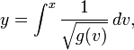
To be simple, if variance of X is function of mean, V(X)=g(u), where u is mean of variable X (e.g. u=E(X)), then the proper VST is:

For example, the Anscombe transform is to transform Poisson distribution (where u=v) to Gaussian distribution:

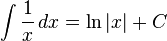
If V(X)=g(u)=u^2, then the integration of 1/x is log(x). 

That's what we usually used for microarray, RNAseq transformation. But do we test the V(X)=u^2 relationship?

We can test the homoskedasticity of residual by Breusch–Pagan test. bptest {lmtest} is the R function. Here is the example output:

> library('lmtest')
> ## generate a regressor
> x <- rep(c(-1,1), 50)
> ## generate heteroskedastic and homoskedastic disturbances
> err1 <- rnorm(100, sd=rep(c(1,2), 50))
> err2 <- rnorm(100)
> ## generate a linear relationship
> y1 <- 1 + x + err1
> y2 <- 1 + x + err2
> ## perform Breusch-Pagan test
> bptest(y1 ~ x)
studentized Breusch-Pagan test
data:  y1 ~ x
BP = 15.867, df = 1, p-value = 6.795e-05
> bptest(y2 ~ x)
studentized Breusch-Pagan test
data:  y2 ~ x
BP = 7e-04, df = 1, p-value = 0.9784

y1 is significantly heteroskedastic, because the p-value is <0.05.